In the previous post, we covered word embeddings: how every word (and every sentence) can be represented as a list of numbers, a vector, that captures its meaning. Similar words end up with similar vectors. Different words end up with different vectors.
But that raises an obvious next question: how do you actually measure how similar two vectors are?
Before answering that, it's worth pausing on why this question matters so much right now. Measuring the similarity between embeddings is not an academic exercise. It is the core operation behind two of the most widely used AI capabilities in production today.
Semantic search works by converting a user's query into a vector, converting every document in a collection into vectors, and finding the documents whose vectors are most similar to the query vector. Every time you search by meaning rather than exact keywords, embedding similarity is what's running underneath.
RAG (Retrieval-Augmented Generation) works the same way. When an AI assistant retrieves relevant context before generating an answer, it does so by computing similarity between the query embedding and thousands of stored document embeddings, then passing the closest matches to the language model. The quality of that retrieval determines the quality of the answer.
This is live, production-grade technology running in search engines, AI assistants, recommendation systems, and document databases right now. Understanding how it works starts here.
If you have the vector for "dog" and the vector for "cat," how do you turn those two lists of numbers into a single score that tells you how close in meaning they are? And how is that different from the vector for "dog" and "aeroplane," which should score much lower?
That's what this post is about. We're going to cover the main ways NLP systems measure similarity and distance between vectors and text. Some of these you'll use directly when building semantic search or RAG systems. Others are foundational concepts that help you understand what's happening under the hood.
The most important one, the one that powers most of modern NLP, is cosine similarity. But we'll also cover the alternatives, when each one makes sense, and how they compare.
What Is Vector Similarity?
Before getting into specific methods, let's make sure the core idea is clear.
A vector is just a list of numbers. In NLP, every word or sentence gets converted into a vector by a model like Word2Vec or BERT. Two sentences that mean similar things will have vectors that are numerically similar in some way. Two sentences about completely different topics will have vectors that are numerically different.
Vector similarity is the general term for any method that takes two vectors and produces a single score representing how alike they are. A high score means similar. A low score means different.
There are several ways to compute this score, and they each have different properties. The choice between them matters, and we'll explain why as we go through each one.
Cosine Similarity
Cosine similarity is the most widely used similarity metric in NLP. It's the default choice in semantic search systems, recommendation engines, and RAG pipelines. If someone says they're comparing embeddings, they almost certainly mean cosine similarity.
The Intuition
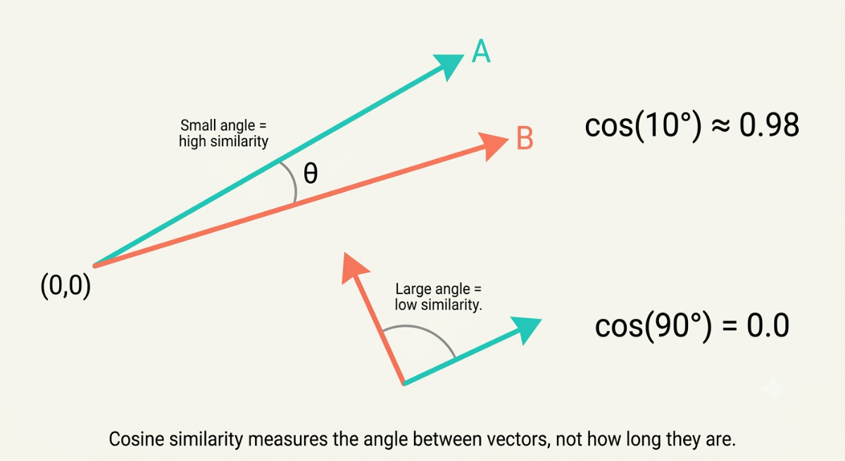
Here's the key insight behind cosine similarity: it measures the angle between two vectors, not the distance between their endpoints.
Imagine two arrows pointing outward from the origin of a graph. If the two arrows point in almost the same direction, the angle between them is small, and the cosine similarity is high (close to 1). If they point in completely different directions, the angle is large, and the cosine similarity is low (close to 0 or even negative).
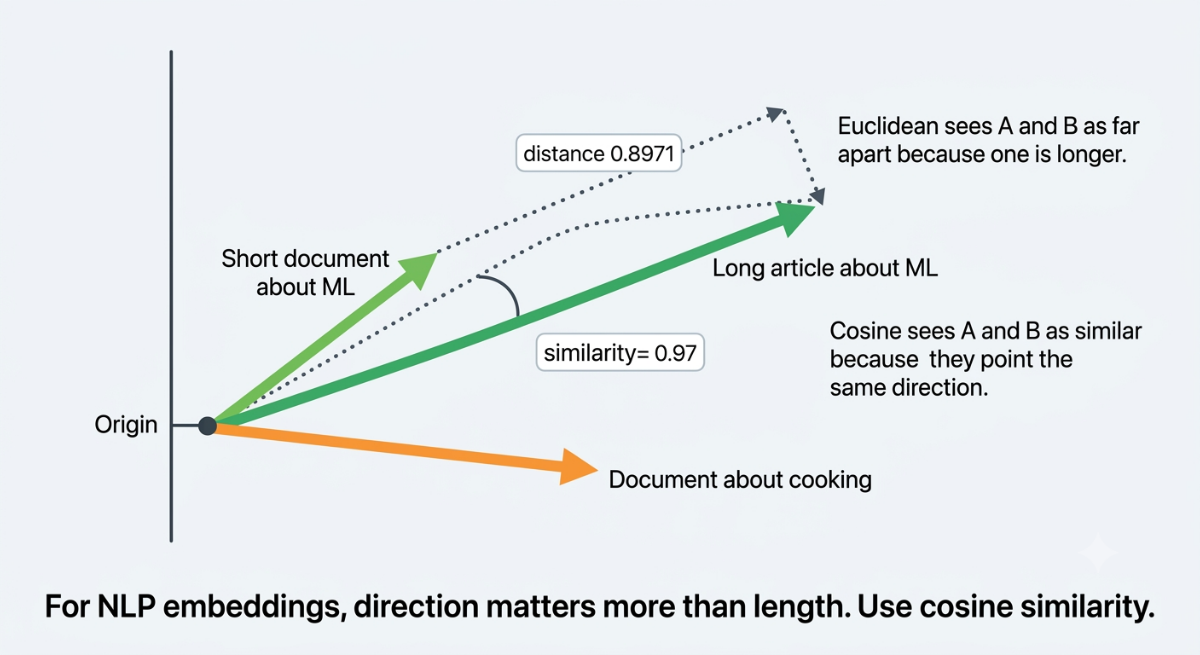
Why does angle matter more than distance? Because in NLP, we care about direction, not magnitude. A short document and a long document about the same topic might have vectors of very different lengths (magnitudes), but they'll point in roughly the same direction. Measuring the angle between them correctly identifies them as similar even though their vector lengths differ.
The Formula
Cosine similarity between two vectors A and B is calculated as:
cosine similarity = (A · B) / (|A| × |B|)
In plain terms: - A · B is the dot product: multiply each pair of corresponding numbers and add them all up - |A| and |B| are the lengths (magnitudes) of each vector: the square root of the sum of squared values - Dividing by the lengths normalises for vector size, so only direction matters
The result is always a number between -1 and 1: - 1.0 means the vectors point in exactly the same direction (identical meaning) - 0.0 means the vectors are perpendicular (no relationship) - -1.0 means the vectors point in opposite directions (opposite meaning)
In practice with word and sentence embeddings, you rarely see negative values. Most scores fall between 0 and 1.
Cosine Similarity in Python
from sklearn.metrics.pairwise import cosine_similarity
from sentence_transformers import SentenceTransformer
import numpy as np

model = SentenceTransformer('all-MiniLM-L6-v2')

sentences = [
    "The cat sat on the mat.",
    "A kitten rested on the rug.",
    "Machine learning is a subset of AI.",
    "I enjoy cooking Italian food."
]

embeddings = model.encode(sentences)
similarity_matrix = cosine_similarity(embeddings)

print(similarity_matrix.round(2))
Output:
[[1.   0.71 0.06 0.09]
 [0.71 1.   0.04 0.11]
 [0.06 0.04 1.   0.05]
 [0.09 0.11 0.05 1.  ]]
Sentences 1 and 2 score 0.71 despite sharing almost no keywords. "Cat" and "kitten" are synonyms. "Sat" and "rested" are related. "Mat" and "rug" are similar objects. The embeddings have captured all of that, and the cosine similarity score reflects it. Sentences 1 and 3, about completely different topics, score 0.06.
Manual Calculation
If you want to understand exactly what's happening, here's the same calculation done manually on two simple two-dimensional vectors:
import numpy as np

# Two simple 2D vectors
a = np.array([1, 2])
b = np.array([2, 3])

# Dot product
dot_product = np.dot(a, b)           # 1*2 + 2*3 = 8

# Magnitudes
magnitude_a = np.linalg.norm(a)      # sqrt(1^2 + 2^2) = sqrt(5) ≈ 2.236
magnitude_b = np.linalg.norm(b)      # sqrt(2^2 + 3^2) = sqrt(13) ≈ 3.606

# Cosine similarity
cos_sim = dot_product / (magnitude_a * magnitude_b)
print(f"Cosine similarity: {cos_sim:.4f}")
# Output: Cosine similarity: 0.9923
Two vectors pointing in very similar directions. Score of 0.99: nearly identical.
What Is Cosine Distance?
Cosine distance is simply 1 minus cosine similarity:
cosine distance = 1 - cosine similarity
It converts the similarity score into a distance score. High similarity (close to 1) becomes low distance (close to 0). Low similarity becomes high distance.
The two terms describe the same relationship from opposite angles. Similarity asks "how alike are these?" Distance asks "how far apart are these?" You'll see both used in different libraries and papers, but they're measuring the same thing.
Euclidean Distance
Euclidean distance is the straight-line distance between two points in space. It's the most natural notion of distance, the kind you learned in school.
For two points in 2D space, it's the length of the line connecting them. In higher dimensions (like the 768-dimensional space of BERT embeddings), the same formula extends naturally: take the difference between each pair of corresponding numbers, square them, add them all up, and take the square root.
import numpy as np

a = np.array([1, 2])
b = np.array([4, 6])

euclidean_distance = np.linalg.norm(a - b)
print(f"Euclidean distance: {euclidean_distance:.4f}")
# Output: Euclidean distance: 5.0000
Cosine Similarity vs Euclidean Distance
So which one should you use?
For NLP tasks with word and sentence embeddings, cosine similarity almost always performs better. Here's why.
Imagine you have two documents about machine learning. One is a short tweet (50 words) and one is a long article (2000 words). Both are about the same topic, so their embedding vectors should point in roughly the same direction. But the article's vector might be much longer (larger magnitude) simply because it represents more text.
Cosine similarity ignores magnitude and only looks at direction. It correctly identifies both documents as similar. Euclidean distance would penalise the difference in vector length and potentially rate them as dissimilar just because one is longer.
Use Euclidean distance when the magnitude of vectors genuinely carries information you care about. In most NLP tasks, it doesn't.
Jaccard Similarity
Jaccard similarity takes a completely different approach. Instead of comparing vectors of numbers, it compares sets of items.
The formula is simple: the size of the overlap between two sets divided by the size of their union.
Jaccard similarity = |A ∩ B| / |A ∪ B|
In plain terms: how many items do these two sets share, divided by the total number of unique items across both sets?
def jaccard_similarity(set_a, set_b):
    intersection = set_a & set_b
    union = set_a | set_b
    return len(intersection) / len(union)

doc1 = set(["the", "cat", "sat", "on", "the", "mat"].split() if isinstance("the", str) else ["the", "cat", "sat", "on", "mat"])
doc2 = set(["the", "cat", "sat", "on", "the", "hat"])
doc3 = set(["the", "dog", "ran", "in", "the", "park"])

doc1_words = {"the", "cat", "sat", "on", "mat"}
doc2_words = {"the", "cat", "sat", "on", "hat"}
doc3_words = {"the", "dog", "ran", "in", "park"}

print(f"Doc1 vs Doc2: {jaccard_similarity(doc1_words, doc2_words):.2f}")
print(f"Doc1 vs Doc3: {jaccard_similarity(doc1_words, doc3_words):.2f}")
Output:
Doc1 vs Doc2: 0.67
Doc1 vs Doc3: 0.17
Documents 1 and 2 share "the," "cat," "sat," "on" (4 words) out of 6 unique words total, giving 4/6 ≈ 0.67. Documents 1 and 3 only share "the" (1 word) out of 9 unique words, giving 1/9 ≈ 0.11.
Jaccard similarity is useful for comparing short texts, sets of tags or labels, or any situation where you care about overlap between items rather than semantic similarity. It's commonly used in deduplication (finding near-duplicate documents) and in recommendation systems that compare sets of user preferences. It works purely on word overlap and knows nothing about meaning, so it won't help you find that "automobile" and "car" are related.
Edit Distance and Levenshtein Distance
So far, all the methods we've looked at operate on whole words or vectors. Edit distance operates at the character level, which makes it useful for a completely different set of problems.
Edit distance (also called Levenshtein distance, after the Soviet mathematician Vladimir Levenshtein who defined it in 1965) measures how many single-character operations it takes to turn one string into another. The three allowed operations are:
- Insertion: add a character
- Deletion: remove a character
- Substitution: replace one character with another
# Python has no built-in edit distance, but it's straightforward to compute
# or use the python-Levenshtein library

def levenshtein_distance(s1, s2):
    m, n = len(s1), len(s2)
    dp = [[0] * (n + 1) for _ in range(m + 1)]

    for i in range(m + 1):
        dp[i][0] = i
    for j in range(n + 1):
        dp[0][j] = j

    for i in range(1, m + 1):
        for j in range(1, n + 1):
            if s1[i-1] == s2[j-1]:
                dp[i][j] = dp[i-1][j-1]
            else:
                dp[i][j] = 1 + min(dp[i-1][j],    # deletion
                                   dp[i][j-1],    # insertion
                                   dp[i-1][j-1])  # substitution
    return dp[m][n]

print(levenshtein_distance("kitten", "sitting"))   # 3
print(levenshtein_distance("sunday", "saturday"))  # 3
print(levenshtein_distance("cat", "cat"))           # 0
print(levenshtein_distance("cat", "car"))           # 1
Output:
3
3
0
1
"Kitten" to "sitting" takes 3 operations: substitute k with s, substitute e with i, insert g at the end. "Cat" to "car" takes 1 operation: substitute t with r.
When Is Edit Distance Useful?
Edit distance is not for measuring semantic similarity. It has no idea what words mean. "Cat" and "feline" are semantically very similar but have a high edit distance. "Cat" and "car" are semantically unrelated but have an edit distance of just 1.
What edit distance is excellent for:
Spell checking and autocorrect. When someone types "recieve," a spell checker computes edit distance to all dictionary words and suggests "receive" (edit distance 1) as the most likely correction.
Fuzzy string matching. Searching a database for "Smithe, John" when the record says "Smith, John" requires tolerating small character-level differences. Edit distance makes this possible.
DNA sequence alignment. Bioinformatics uses edit distance to measure how similar two genetic sequences are, which is one of its most important applications outside NLP.
Handling typos in user input. Before showing "no results found," a search system can check if the query is close (by edit distance) to known valid terms and suggest the correction.
Choosing the Right Similarity Metric
Here's a practical summary of when to reach for each method:
| Metric | Operates on | Best for |
|---|---|---|
| Cosine similarity | Vectors | Semantic similarity, embedding comparison, semantic search |
| Euclidean distance | Vectors | Clustering when magnitude matters |
| Jaccard similarity | Sets of words | Text overlap, deduplication, tag comparison |
| Edit distance / Levenshtein | Character strings | Spell checking, fuzzy matching, typo tolerance |
The most important takeaway: cosine similarity is the default for anything involving embeddings. When you're working with word vectors, sentence vectors, or document vectors from any modern NLP model, cosine similarity is almost always the right choice.
The other metrics are not inferior. They're designed for different problems. Edit distance is the right tool for spell checking in a way that cosine similarity never could be. Jaccard is perfectly suited for comparing sets of tags. Understanding what each one measures helps you pick the right one.
A Complete Semantic Search Example
Let's put cosine similarity to work in a minimal semantic search system: given a query, find the most relevant documents from a small collection.
from sentence_transformers import SentenceTransformer
from sklearn.metrics.pairwise import cosine_similarity
import numpy as np

model = SentenceTransformer('all-MiniLM-L6-v2')

# Our document collection
documents = [
    "Python is a popular programming language for data science.",
    "Machine learning models learn patterns from training data.",
    "Neural networks are inspired by the structure of the human brain.",
    "Deep learning is a subset of machine learning using many layers.",
    "Natural language processing helps computers understand text.",
    "I enjoy hiking in the mountains on weekends.",
    "The best pasta recipe uses fresh tomatoes and basil."
]

# Encode documents
doc_embeddings = model.encode(documents)

def semantic_search(query, top_k=3):
    query_embedding = model.encode([query])
    scores = cosine_similarity(query_embedding, doc_embeddings)[0]
    top_indices = np.argsort(scores)[::-1][:top_k]

    print(f"Query: '{query}'\n")
    for i, idx in enumerate(top_indices):
        print(f"  {i+1}. Score: {scores[idx]:.3f} | {documents[idx]}")
    print()

semantic_search("how do AI systems learn from examples?")
semantic_search("what is NLP?")
semantic_search("outdoor activities")
Output:
Query: 'how do AI systems learn from examples?'

  1. Score: 0.612 | Machine learning models learn patterns from training data.
  2. Score: 0.521 | Deep learning is a subset of machine learning using many layers.
  3. Score: 0.489 | Neural networks are inspired by the structure of the human brain.

Query: 'what is NLP?'

  1. Score: 0.671 | Natural language processing helps computers understand text.
  2. Score: 0.412 | Machine learning models learn patterns from training data.
  3. Score: 0.387 | Deep learning is a subset of machine learning using many layers.

Query: 'outdoor activities'

  1. Score: 0.482 | I enjoy hiking in the mountains on weekends.
  2. Score: 0.201 | Python is a popular programming language for data science.
  3. Score: 0.187 | Natural language processing helps computers understand text.
Notice that the query "how do AI systems learn from examples?" correctly retrieves the machine learning document without sharing a single keyword with it. The query uses "AI systems" and "learn from examples." The document says "machine learning models" and "patterns from training data." BM25 would score this at zero. Cosine similarity on sentence embeddings scores it at 0.612.
That's the power of embedding-based retrieval.
What Comes Next
You now understand how NLP systems measure similarity: cosine similarity for comparing vectors, Euclidean distance for straight-line gaps, Jaccard for set overlap, and edit distance for character-level matching.
These tools are the foundation of the next set of topics. In the next post, we'll cover Sentiment Analysis: how NLP systems automatically detect whether a piece of text is positive, negative, or neutral, and where that capability is used at scale in the real world.
Learn This at Fondra Labs
This post is part of our NLP Foundations series, where we build up practical AI knowledge one concept at a time, from text processing basics all the way to the systems powering modern AI.
At Fondra Labs, we teach AI from production reality, not hype. Every topic in this series is here because it genuinely matters when you sit down to build something real.
If this was useful, explore the rest of the blog. We cover machine learning, deep learning, NLP, and the practical skills that turn understanding into building.
Frequently Asked Questions

Javier Aguirre
Teaching AI from production reality, not hype.
Build your AI Foundations
Get the free checklist that production engineers use to avoid these common RAG pitfalls.
Get the Free Guide