In the last post, we covered TF-IDF: the foundational technique for turning text into numbers and scoring how relevant a word is to a document. If you haven't read that one yet, it's worth doing first. BM25 builds directly on those ideas, and the motivation for it becomes much clearer once you've seen what TF-IDF gets right and where it falls short.
Here's a quick recap of where we left off.
TF-IDF scores a word by multiplying two things together: how often it appears in a document (term frequency), and how rare it is across the entire collection (inverse document frequency). The result is a weight that rewards distinctive words and discounts common ones. It works well. It's been used in real search systems for decades.
But it has two specific problems that become hard to ignore when you're building anything at scale.
The first problem: TF-IDF has no ceiling on term frequency. If a document mentions the word "python" twice, it scores higher than one that mentions it once. Fine. But if a document mentions "python" fifty times, it scores twenty-five times higher than the document that mentions it once. At some point, more repetitions stop adding meaningful evidence that a document is relevant. The relationship isn't linear, but TF-IDF treats it as if it is.
The second problem: TF-IDF doesn't handle document length well. A long document will naturally contain more words, including more repetitions of relevant terms, than a short one. That gives longer documents a systematic advantage in raw TF scores, even if the shorter document is actually more focused and relevant.
BM25 was designed to fix both of these problems. It takes the same core intuition as TF-IDF (score documents based on term frequency and rarity) but adds two refinements that make it significantly more robust in practice. Those refinements are what we'll spend most of this post unpacking.
What Is Information Retrieval?
Before getting into BM25 specifically, it helps to place it in context.
Information retrieval is the field concerned with finding relevant material from a large collection in response to a query. It's what a search engine does. You type a question or a set of keywords, and the system returns a ranked list of documents it believes are most relevant to what you asked.
The core challenge in information retrieval is ranking: given a query and a large collection of documents, how do you decide which documents to return, and in what order?
Ranking algorithms take a query and a document and produce a score. Higher score means more relevant. The entire ranked list is built by scoring every candidate document and sorting them. The quality of the search experience depends almost entirely on how good that scoring function is.
TF-IDF was one of the earliest practical scoring functions. BM25 is its direct successor, and it remains the most widely used lexical retrieval algorithm in production systems today.
Lexical retrieval refers to retrieval based on matching the actual words in the query against the actual words in the documents. No semantic understanding is involved. If the query says "python tutorial" and a document contains the words "python" and "tutorial," that document gets a score. If a document covers the same topic but uses the phrase "programming language guide," it may score much lower or not at all, because the words don't overlap.
Lexical retrieval is the category that both TF-IDF and BM25 belong to. It is fast, transparent, and very effective when users search using the same terminology that appears in the documents. Its limitations are the motivation for semantic and hybrid retrieval approaches, which we'll get to later in this series.
What Is BM25?
BM25 stands for Best Match 25. The "25" refers to the fact that it was the 25th iteration in a series of retrieval functions developed through the Okapi research project at City University London in the 1980s and 1990s. You will sometimes see it called Okapi BM25 after that project. The name has stuck.
The BM25 algorithm scores a document against a query by looking at each query term individually, scoring the document for each term, and summing those scores. If your query is "machine learning tutorial," BM25 computes a score for "machine," a score for "learning," and a score for "tutorial," then adds them together to get the document's final relevance score.
The score for each individual term is where the interesting work happens.
The BM25 Formula
Let's build up the formula in pieces, because each piece has a clear purpose.
The full BM25 score for a single query term in a document is:
score(term, document) = IDF(term) × [ TF(term, document) × (k1 + 1) ] / [ TF(term, document) + k1 × (1 - b + b × (doc_length / avg_doc_length)) ]If we display it in a mathematical formula it would be written as follows:
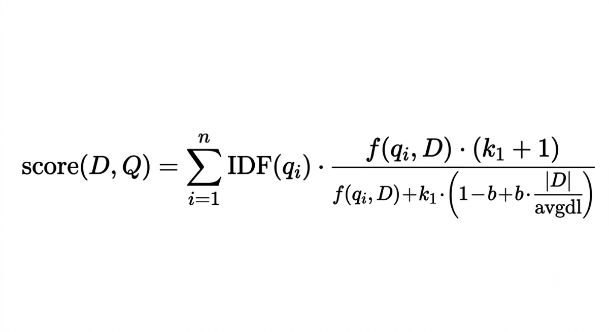
That looks intimidating. It isn't, once you see what each part does. Also, remember, for AI engineering knowing the mathematics is not as important as understanding the underlaying behaviours. Therefore, let me guide you through the general understanding of it.
The IDF Part
The IDF component in BM25 works similarly to TF-IDF. It measures how rare the term is across the entire collection. Rare terms that appear in only a few documents get high IDF scores. Common terms that appear everywhere get low scores.
The exact formula used for IDF varies slightly across implementations, but the principle is the same as in TF-IDF. We won't dwell on it here because you already understand it from the previous post.
The TF Part: Saturation
This is the first of BM25's two key improvements.
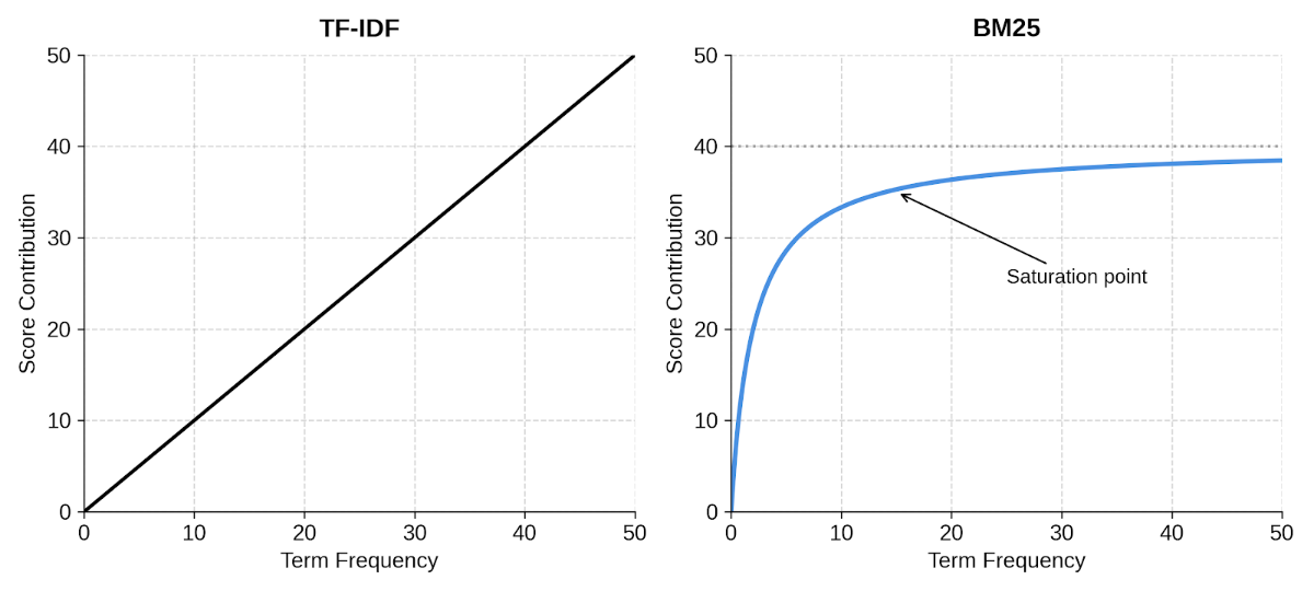
In TF-IDF, the term frequency contribution grows linearly and without limit. In BM25, the contribution of term frequency saturates as the count increases. The 5th occurrence of a word adds meaningful evidence of relevance. The 50th occurrence adds very little on top of that.
The saturation is controlled by a parameter called k1. In practice, k1 is typically set between 1.2 and 2.0.
When k1 is high, the saturation kicks in slowly: more repetitions keep adding score for longer. When k1 is low, the function saturates quickly and additional repetitions matter very little.
Let's see what this looks like concretely. Suppose k1 = 1.5 and ignore length normalisation for now.
| TF (count) | TF-IDF contribution | BM25 TF contribution |
|---|---|---|
| 1 | 1.0 | 0.83 |
| 2 | 2.0 | 1.20 |
| 5 | 5.0 | 1.56 |
| 10 | 10.0 | 1.71 |
| 50 | 50.0 | 1.94 |
The TF-IDF contribution grows without limit. The BM25 contribution approaches a ceiling (around 2.0 with k1 = 1.5) and never exceeds it. A document that mentions a term fifty times is not scored fifty times higher than one that mentions it once. That's a much more realistic model of relevance.
The Length Normalisation Part
This is BM25's second key improvement.
A long document will naturally repeat terms more often than a short one, just by virtue of having more words. TF-IDF doesn't account for this at all. BM25 adjusts for it by comparing each document's length to the average document length across the collection.
This adjustment is controlled by a parameter called b, typically set around 0.75.
When b = 1.0, full length normalisation is applied: longer documents are penalised proportionally. When b = 0, no length normalisation is applied, and BM25 behaves more like TF-IDF in this respect. In practice, b = 0.75 provides a partial normalisation: long documents are penalised somewhat, but not to the point where a genuinely comprehensive document is dismissed just for being thorough.
The intuition is: if a short document and a long document both mention a query term the same number of times, the short document is probably more focused on that topic. BM25 rewards that focus.
A Worked Example
Let's make this concrete with the same setup used in the previous post: a collection of 1,000 news articles, and a query for the word "candidacy."
Suppose we have two documents:
Document A (120 words): mentions "candidacy" 3 times. Document B (600 words): mentions "candidacy" 8 times.
Which document should rank higher for the query "candidacy"?
Intuitively, Document A is probably more focused on the topic. It's short, and "candidacy" appears three times in just 120 words. Document B mentions it more often in absolute terms, but it's a much longer piece where the term is less central.
TF-IDF would give Document B a higher raw score just because of the higher count. BM25 adjusts for both the diminishing returns of higher counts and the longer document length.
Let's assume the average document length in the collection is 300 words, k1 = 1.5, and b = 0.75.
For Document A (3 occurrences, 120 words):
Length ratio = 120 / 300 = 0.4
Length adjustment = 1 - 0.75 + 0.75 × 0.4 = 0.55
TF contribution = (3 × 2.5) / (3 + 1.5 × 0.55) = 7.5 / 3.825 ≈ 1.96
For Document B (8 occurrences, 600 words):
Length ratio = 600 / 300 = 2.0
Length adjustment = 1 - 0.75 + 0.75 × 2.0 = 1.75
TF contribution = (8 × 2.5) / (8 + 1.5 × 1.75) = 20 / 10.625 ≈ 1.88
Document A scores slightly higher than Document B, despite fewer raw mentions. The shorter, more focused document wins. That's the behaviour we wanted.
BM25 in Python
There is no BM25 in scikit-learn, but several reliable libraries implement it. The most commonly used is `rank_bm25`.
pip install rank-bm25Here's a minimal working example:
from rank_bm25 import BM25Okapi

# Your documents, pre-tokenized (split into word lists)
documents = [
    "machine learning algorithms learn patterns from data".split(),
    "deep learning uses neural networks with many layers".split(),
    "natural language processing handles text and speech".split(),
    "computer vision processes images and video".split(),
    "neural networks are inspired by the human brain".split()
]

# Build the BM25 index
bm25 = BM25Okapi(documents)

# Query
query = "neural networks deep learning".split()

# Get scores for each document
scores = bm25.get_scores(query)
print(scores)

# Get the top N most relevant documents
top_docs = bm25.get_top_n(query, documents, n=2)
for doc in top_docs:
    print(" ".join(doc))
Output:
[0.    2.31  0.    0.    1.84]
deep learning uses neural networks with many layers
neural networks are inspired by the human brain
A few things worth noting here.
The documents are passed as lists of tokens, not raw strings. That means you handle tokenization yourself before passing anything to BM25. In practice this is a feature, not a limitation: it means you can apply any preprocessing you want first (lowercasing, stemming, stop word removal, domain-specific tokenization) before the BM25 index sees the text.
You can also adjust k1 and b directly:
bm25 = BM25Okapi(documents, k1=1.2, b=0.8)A More Realistic Example
In practice, you'd want to preprocess your text before indexing. Here's a slightly more complete pipeline:
from rank_bm25 import BM25Okapi
import re

def tokenize(text):
    # Lowercase and split on non-alphanumeric characters
    return re.findall(r'\b[a-z]+\b', text.lower())

raw_documents = [
    "Machine learning algorithms learn patterns from data",
    "Deep learning uses neural networks with many layers",
    "Natural language processing handles text and speech",
    "Computer vision processes images and video",
    "Neural networks are inspired by the human brain"
]

tokenized_docs = [tokenize(doc) for doc in raw_documents]
bm25 = BM25Okapi(tokenized_docs)

query_tokens = tokenize("neural networks and deep learning")
scores = bm25.get_scores(query_tokens)

ranked = sorted(zip(scores, raw_documents), reverse=True)
for score, doc in ranked:
    print(f"{score:.3f} — {doc}")
Output:
2.312 — Deep learning uses neural networks with many layers
1.843 — Neural networks are inspired by the human brain
0.000 — Machine learning algorithms learn patterns from data
0.000 — Natural language processing handles text and speech
0.000 — Computer vision processes images and video
The same two documents come out on top as in the TF-IDF example from the previous post, which makes sense: the query terms overlap with those documents. The difference is in how the scoring behaves as documents get longer or repeat terms more.
Why NLP Fundamentals Pay Off Here
The tokenization in the example above is deliberately simple: lowercase and split on whitespace. In a real system, the preprocessing step is where everything we've covered earlier in this series starts earning its keep.
BM25 scores what it receives. The quality of retrieval depends heavily on the quality of the tokens you feed into it. That means the linguistic techniques from earlier posts aren't abstract exercises. They're practical inputs to a better search index.
Here's how several of them connect directly to BM25:
Tokenization is the foundation. Every token becomes a term in the index. Poor tokenization (splitting on whitespace only, failing to handle punctuation, not lowercasing consistently) introduces noise that degrades matching. A query for "run" and a document containing "Run." may not match if normalisation wasn't applied.
Lemmatization and stemming collapse inflected forms of a word into a common base. Without them, "run," "runs," "running," and "ran" are four different terms in the index. A query for "running" won't match a document that only says "ran." With lemmatization, all four map to "run" and matching improves significantly.
Stop word removal eliminates high-frequency words that carry little retrieval value: "the," "a," "is," "on." Removing them reduces index size and prevents these terms from consuming scoring weight that should go to meaningful content words.
POS tagging doesn't improve BM25 directly, but it enables smarter filtering decisions. If you know which tokens are nouns, verbs, and adjectives, you can make deliberate choices: keep only content words, remove function words that stop word lists miss, or apply different normalisation strategies to different parts of speech. Better filtering leads to a cleaner index, and a cleaner index leads to better retrieval scores.
The gains compound. A BM25 system built on top of careful tokenization, lemmatization, stop word removal, and POS-informed filtering will consistently outperform one built on raw whitespace splitting, using the same scoring parameters and the same documents.
Multilingual systems take this further
Language-specific preprocessing becomes especially important when working outside English. Korean, for example, attaches grammatical particles such as 는, 은, 이, and 가 directly to words. Without morphological analysis, a query and a document may refer to exactly the same concept but appear as completely different surface forms. No amount of BM25 parameter tuning fixes a vocabulary mismatch that happens before the scoring function ever runs.
Similar considerations exist for Japanese (word segmentation), Chinese (character vs. word tokenization), German (compound word splitting), Arabic (root-based morphology), and many other languages. In each case, the preprocessing layer, informed by the linguistic structure of the language, is what allows BM25 to function well.
This is one of the clearest demonstrations that NLP fundamentals continue to matter even when working with relatively simple retrieval algorithms. The preprocessing stack and the scoring function are not separate concerns. They are two parts of the same system, and the quality of one directly determines the ceiling of the other.
Both methods score documents based on term frequency and inverse document frequency. The difference is in the details of the TF component.
| Property | TF-IDF | BM25 |
|---|---|---|
| Term frequency growth | Linear, unbounded | Saturates toward a ceiling |
| Document length handling | None (or basic normalisation) | Explicit, tunable via b |
| Tunable parameters | None | k1 (saturation), b (length normalisation) |
| Typical use today | Feature extraction, classification | Search ranking, retrieval |
For text classification and feature extraction tasks, TF-IDF is still the standard choice. Its simplicity and compatibility with scikit-learn's ecosystem make it practical and easy to work with.
For search and ranking tasks (where you're scoring documents against queries and returning a ranked list) BM25 is the better default. Its saturation and length normalisation make it more robust to the kinds of variation you see in real document collections.
Where BM25 Fits in Real Systems
BM25 is not just a theoretical improvement over TF-IDF. It is the default ranking function in Elasticsearch and OpenSearch, two of the most widely deployed search platforms in the world. When a developer sets up a full-text search index without configuring a custom scorer, BM25 is what's running underneath.
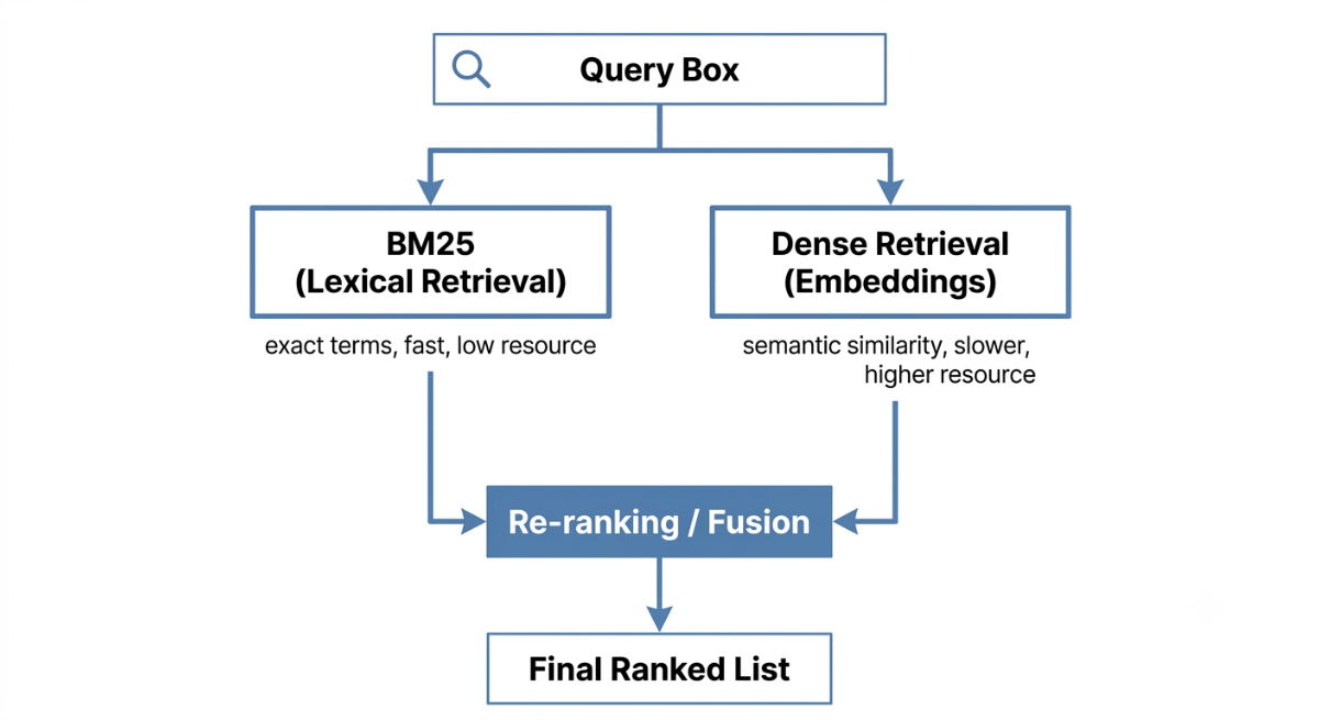
It's also the sparse retrieval component in most hybrid search architectures. A hybrid search system typically runs two retrieval steps in parallel: a BM25 step that matches exact keywords quickly, and a dense neural retrieval step that finds semantically similar documents even when the vocabulary doesn't overlap. The results from both steps are then combined and re-ranked.
This combination exists because BM25 and dense retrieval are genuinely complementary. BM25 is extremely fast and reliable for exact keyword matching. It handles queries with rare, specific terminology (product codes, names, technical terms) very well. Dense retrieval handles conceptual similarity and synonym matching better, but is slower and more resource-intensive. Neither is strictly better than the other. Production systems that care about search quality tend to use both.
The practical takeaway: if you are building anything involving search over text, BM25 is the right starting point for the lexical component. It is well-understood, well-supported, fast, and transparent. You can inspect its scores, tune its parameters, and reason about why a particular document ranked where it did. That interpretability is valuable, especially in early development.
The Limits of Lexical Retrieval
BM25 improves on TF-IDF in important ways, but it is still fundamentally a lexical retrieval method. It matches words. It does not understand meaning.
If a user searches for "heart attack symptoms" and a document discusses "myocardial infarction warning signs," BM25 will likely score that document low. The terms don't overlap. A dense retrieval system trained on medical text would probably find it.
This is the core limitation that motivates the move toward semantic and dense retrieval methods. BM25 gets you very far. It is reliable, efficient, and handles the majority of real-world queries well. But for queries that require understanding synonyms, paraphrases, or conceptual relationships, you need something beyond lexical matching.
That's where word embeddings come in. In the next post, we'll cover how words get represented as dense vectors that capture something closer to meaning, and how that opens the door to a fundamentally different kind of retrieval.
Learn This at Fondra Labs
This post is part of our NLP Foundations series, where we build up practical AI knowledge one concept at a time, from text processing basics all the way to the systems powering modern AI.
At Fondra Labs, we teach AI from production reality, not hype. Every topic in this series is here because it genuinely matters when you sit down to build something real.
If this was useful, explore the rest of the blog. We cover machine learning, deep learning, NLP, and the practical skills that turn understanding into building.
Frequently Asked Questions

Javier Aguirre
Teaching AI from production reality, not hype.
Build your AI Foundations
Get the free checklist that production engineers use to avoid these common RAG pitfalls.
Get the Free Guide